Tutorial

This page demonstrates the Python frontend of Bench-MR.

Construct MPB Instance

The MPB class exposes the settings and several helper functions of an experiment that runs on a single CPU. A single experiment can consist of multiple runs in different environments of the same type, using a set of predefined planners, steer functions, and post-smoothing methods.

from mpb import MPB
mpb = MPB()

The MPB instance is created via the following constructor:

mpb = MPB(config_file = os.path.join(MPB_BINARY_DIR, 'benchmark_template.json'),
          output_path = '')

Argument	Description
config_file	Path name of the configuration JSON file this experiment is based on
output_path	Path where the resulting log files are stored from this experiment

Configuration

Any configuration values (or subtrees) can be set and retrieved using the bracket operator on the MPB instance. The key is a string and by using the dot-notation, a path can be given:

mpb["ompl.seed"] = 4  # set the seed of the OMPL planners

Some helper functions are available to set environment properties, and configure the planners, steer functions and post smoothers:

mpb.set_corridor_grid_env(radius = 3)
mpb.set_planners(['rrt', 'rrt_star', 'informed_rrt_star'])
mpb.set_steer_functions(['reeds_shepp'])

Run the motion planning benchmark:

mpb.run(id='test_run', runs=3)  # optional run ID, number of runs (environments)

The following command summarizes some basic planning results from these 3 runs that were just executed:

mpb.print_info()

+++++++++++++++++++++++++ Run #0 (1 / 3) +++++++++++++++++++++++++
+ Steering:        Reeds-Shepp 
+ Environment:     grid
+ Planners:        RRT, RRTstar, InformedRRTstar
+ Found solution:  3 / 3
+ Exact solution:  3 / 3
+ Found colliding: 0 / 3
++++++++++++++++++++++++++++++++++++++++++++++++++++++++++++++++++

+++++++++++++++++++++++++ Run #1 (2 / 3) +++++++++++++++++++++++++
+ Steering:        Reeds-Shepp 
+ Environment:     grid
+ Planners:        RRT, RRTstar, InformedRRTstar
+ Found solution:  3 / 3
+ Exact solution:  3 / 3
+ Found colliding: 0 / 3
++++++++++++++++++++++++++++++++++++++++++++++++++++++++++++++++++

+++++++++++++++++++++++++ Run #2 (3 / 3) +++++++++++++++++++++++++
+ Steering:        Reeds-Shepp 
+ Environment:     grid
+ Planners:        RRT, RRTstar, InformedRRTstar
+ Found solution:  3 / 3
+ Exact solution:  3 / 3
+ Found colliding: 0 / 3
++++++++++++++++++++++++++++++++++++++++++++++++++++++++++++++++++

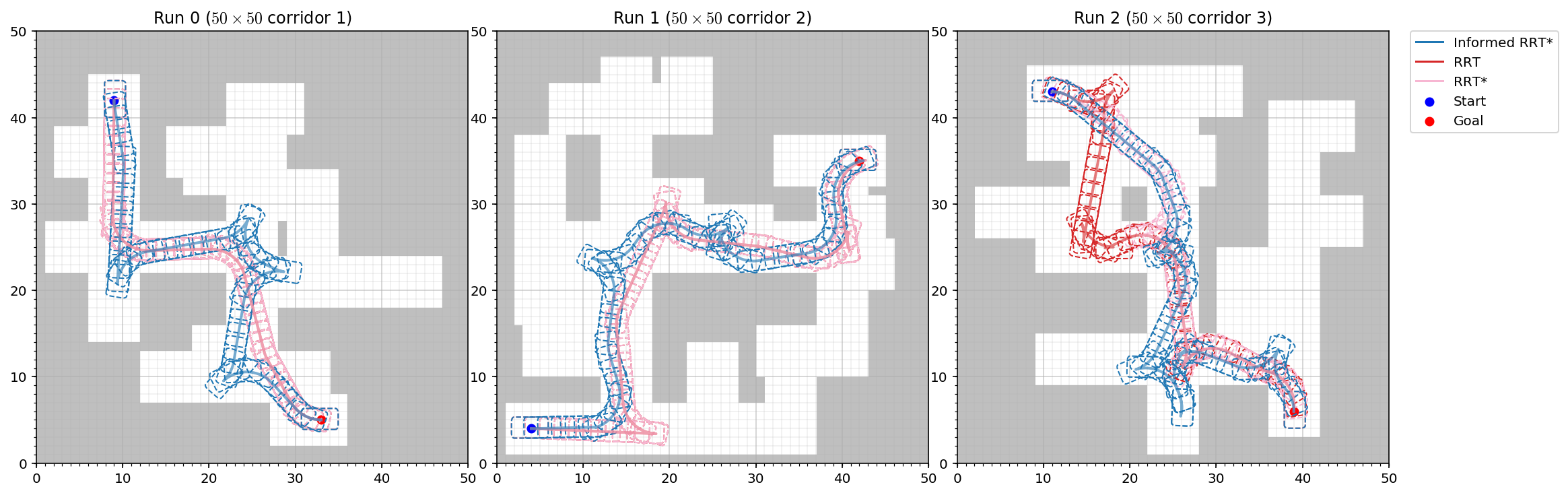
Visualize Trajectories

Visualize the planner trajectories:

mpb.visualize_trajectories()

png

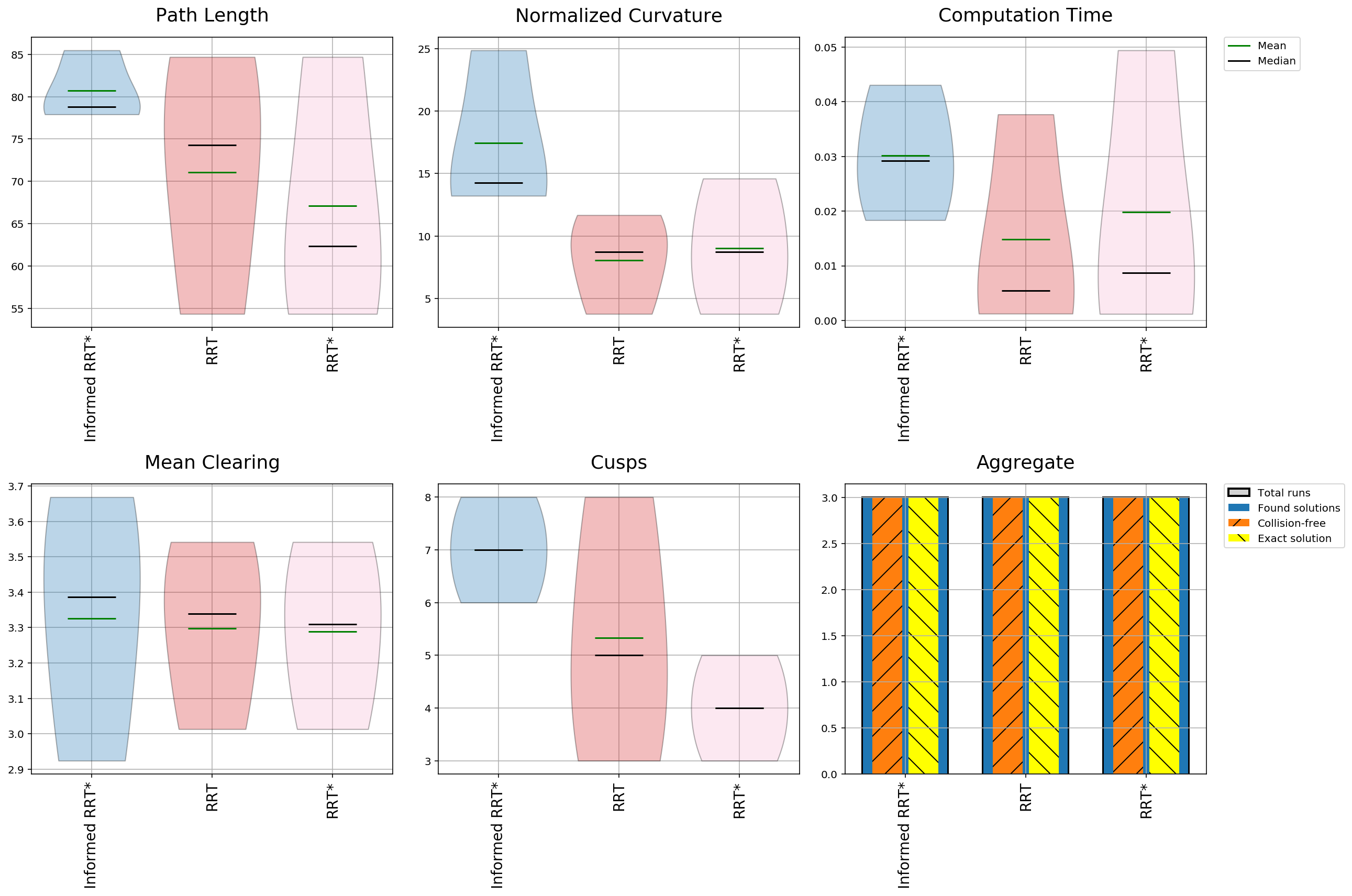
Plot Statistics

Plot planner statistics:

mpb.plot_planner_stats()

png

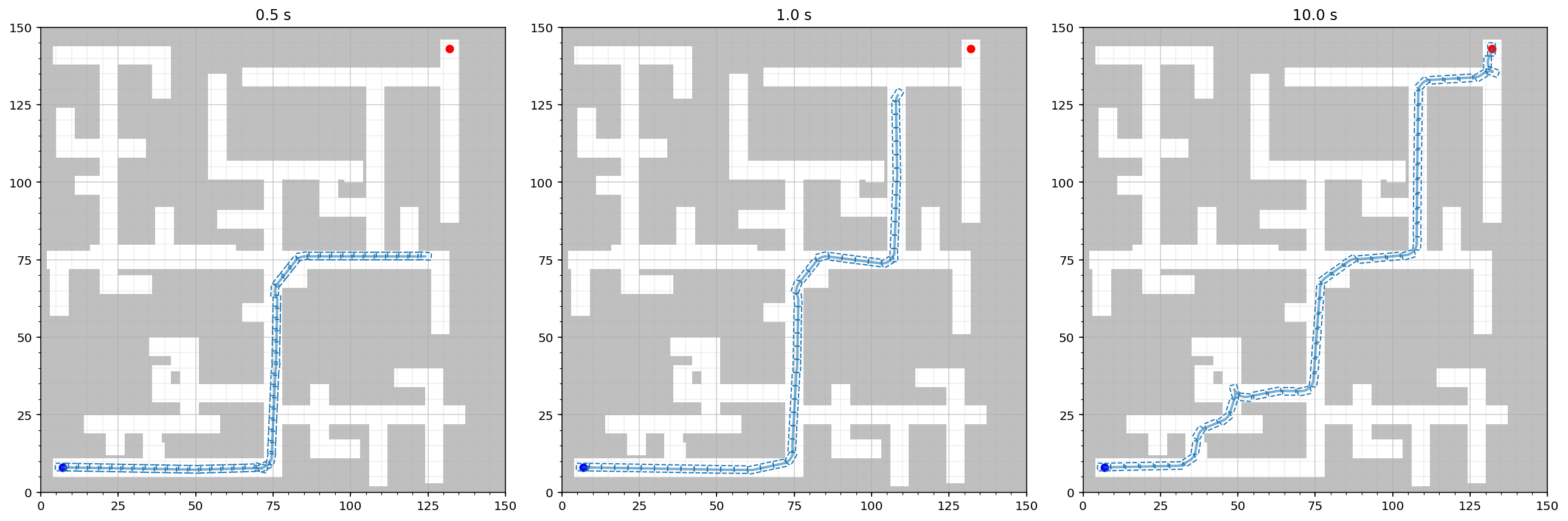
We can also use the frontend to compare the solutions of the anytime planners over the course of a given time interval. Let’s take an Informed RRT* planner and run it on the time allotments of 0.5s, 1s and 10s:

ms = []
for time in [.5, 1, 10]:
    m = MPB()    
    m["max_planning_time"] = time
    m.set_corridor_grid_env(width=150, height=150, branches=100, radius=3)
    m.set_planners(['informed_rrt_star'])
    m.set_steer_functions(['reeds_shepp'])
    m.run('anytime_%.1f' % time, runs=1)
    ms.append(m)    

Visualize the results:

plt.figure(figsize=(6 * len(ms), 6))
for i, m in enumerate(ms):
    plt.subplot(1, len(ms), i+1)
    m.visualize_trajectories(headless=True, combine_views=False,
                             use_existing_subplot=True, show_legend=False)
    plt.title("%.1f s" % m["max_planning_time"])
plt.tight_layout()
plt.savefig("informed_rrt_star_anytime.pdf")

png

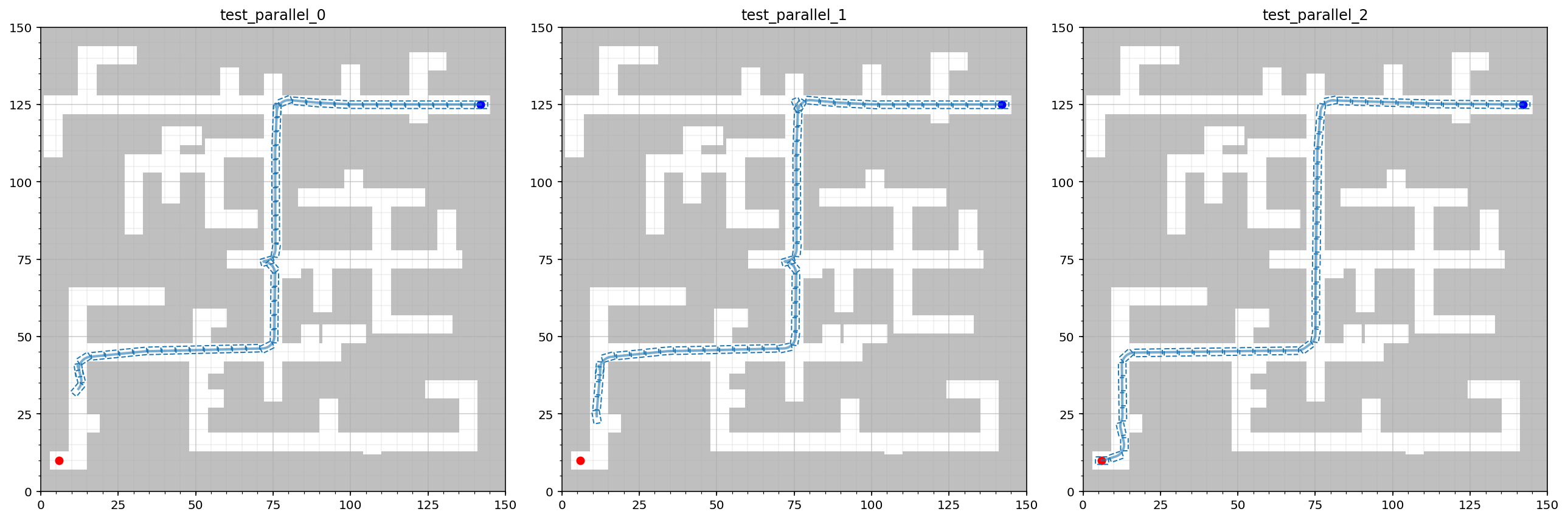
Parallel Execution

Multiple benchmarks can also be run in parallel using MultipleMPB:

from mpb import MultipleMPB

pool = MultipleMPB()
for time in [.5, 1, 10]:
    m = MPB()    
    m["max_planning_time"] = time
    m.set_corridor_grid_env(width=150, height=150, branches=100, radius=3)
    m.set_planners(['informed_rrt_star'])
    m.set_steer_functions(['reeds_shepp'])
    pool.benchmarks.append(m)
    
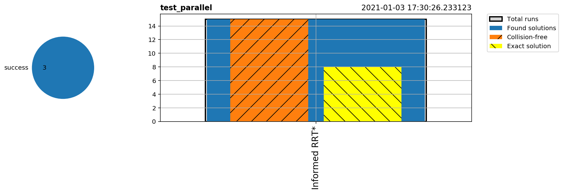
pool.run_parallel('test_parallel', runs=5)

png

pool.visualize_trajectories(run_id='1')

png

View Jupyter Notebook