Grid-based Environments
Load from Image
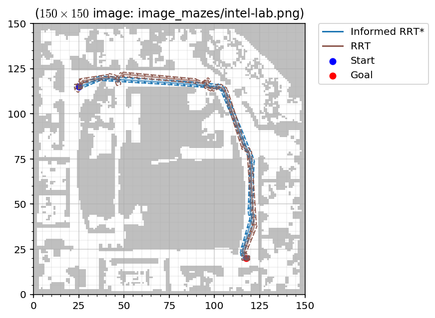
Occupancy grid maps can be loaded from monochromatic images. Based on a defined threshold, darker pixels become occupied grid cells, brighter pixels become unoccupied grid cells. The grid can optionally be scaled (while maintaining its original aspect ratio in case just one desired dimension is given).
MPB.set_image_grid_env(filename: str,
                       desired_width: int = 0,
                       desired_height: int = 0,
                       occupancy_threshold: float = 0.5)
| Argument | Description |
|---|---|
| filename | Filename of the image |
| desired_width | Desired number of horizontal grid cells (keep unchanged if zero) |
| desired_height | Desired number of vertical grid cells (keep unchanged if zero) |
| occupancy_threshold | Pixels with luminance less than this threshold are considered occupied cells |
Example
mpb.set_image_grid_env("image_mazes/intel-lab.png",
                       desired_width=300 * 0.5,
                       desired_height=300 * 0.5,
                       occupancy_threshold=0.98)
mpb.set_planners(['rrt', 'informed_rrt_star'])
mpb.set_steer_functions(['reeds_shepp'])
mpb.set_start(50 * 0.5, 230 * 0.5, 0)
mpb.set_goal(235 * 0.5, 40 * 0.5, 0)
mpb.run(id='test_run_intel', runs=1)
mpb.visualize_trajectories(fig_width=5, fig_height=5)
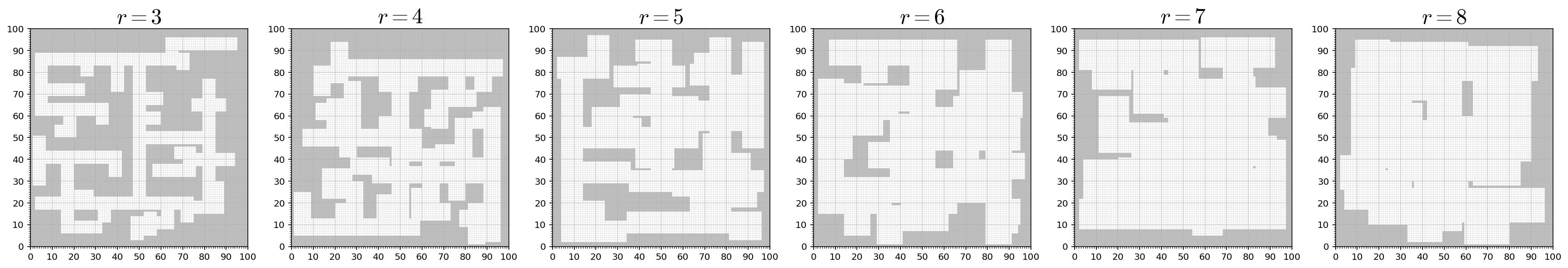
Procedurally Generated Corridors
Corridor-like environments get generated procedurally via the RRT algorithm that extends the current 2D position in either a vertical or a horizontal direction. The resulting tree is created for a defined number of branches and cells within a given radius are set to unoccupied. The cells at the grid boundary are always occupied.
MPB.set_corridor_grid_env(width: int = 50,
                          height: int = 50,
                          branches: int = 40,
                          radius: float = 3.,
                          seed: int = 1)
| Argument | Description |
|---|---|
| width | Number of horizontal grid cells |
| height | Number of vertical grid cells |
| branches | Number of “corridors” to generate (may overlap) |
| radius | Number of cells in both directions horizontally and vertically to free for each generated corridor |
| seed | Seed to use for the random number generator |
Example
parameters = [3, 4, 5, 6, 7, 8]
plt.figure(figsize=(len(parameters) * 5, 5))
for i, parameter in enumerate(parameters):
    plt.subplot(1, len(parameters), i+1)
    m = MPB()
    m.set_corridor_grid_env(100, 100, branches=100, radius=parameter)
    m.set_planners(['informed_rrt_star'])
    m["max_planning_time"] = 1
    m.run(id="corridor", show_progress_bar=False, runs=1)
    run = json.load(open(m.results_filename, "r"))["runs"][0]
    plot_env(run["environment"], draw_start_goal_thetas=False, draw_start_goal=False, set_title=False)
    plt.title("$r = %g$" % parameter, fontsize=24)
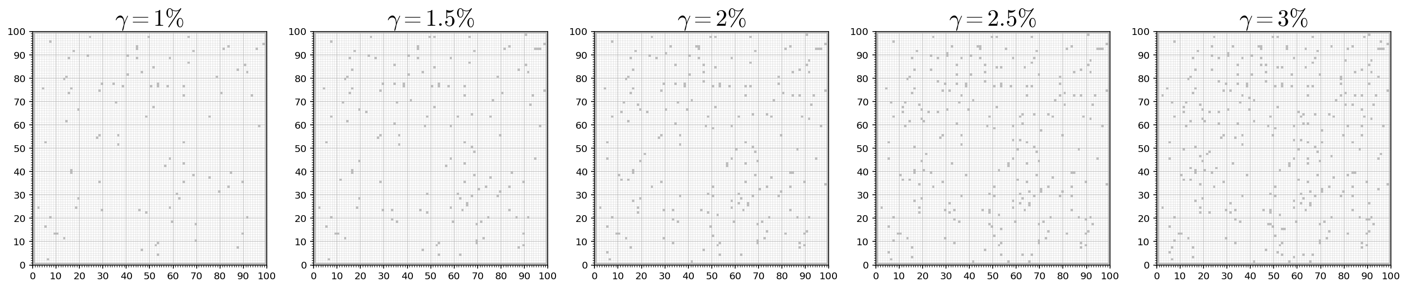
Random Grids
Given a ratio of occupied vs. unoccupied grid cells, grid environments can be randomly generated. The cells at the grid boundary are always occupied.
MPB.set_random_grid_env(width: int = 50,
                        height: int = 50,
                        obstacle_ratio: float = 0.1,
                        seed: int = 1):
| Argument | Description |
|---|---|
| width | Number of horizontal grid cells |
| height | Number of vertical grid cells |
| obstacle_ratio | Fraction of cells to be occupied relative to the total number of cells in the grid |
| seed | Seed to use for the random number generator |
Example
parameters = [0.01, 0.015, 0.02, 0.025, 0.03]
plt.figure(figsize=(len(parameters) * 5, 5))
for i, parameter in enumerate(parameters):
    plt.subplot(1, len(parameters), i+1)
    m = MPB()
    m.set_random_grid_env(100, 100, obstacle_ratio=parameter)
    m.set_planners(['informed_rrt_star'])
    m["max_planning_time"] = 1
    m.run(id="corridor", show_progress_bar=False, runs=1)
    run = json.load(open(m.results_filename, "r"))["runs"][0]
    plot_env(run["environment"], draw_start_goal_thetas=False, draw_start_goal=False, set_title=False)
    plt.title("$\gamma = %g \%%$" % (parameter * 100), fontsize=24)
plt.savefig("obstacle_ratios.pdf", bbox_inches='tight')
# plt.savefig("obstacle_ratios.png", bbox_inches='tight')