Polygon-based Environments
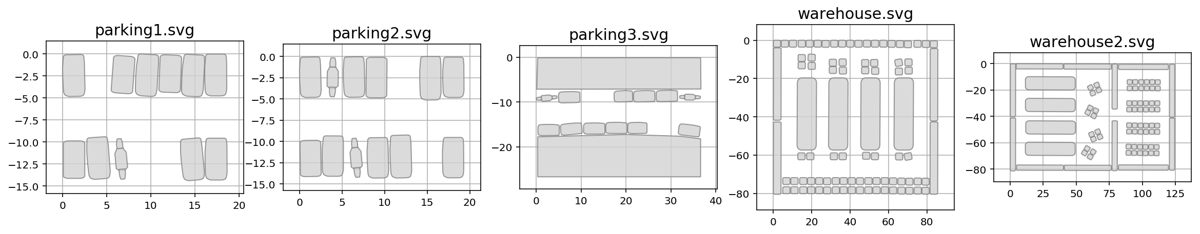
Mazes of this type consist of convex shapes that are stored as paths in a SVG file. We used Inkscape to provide the following example mazes:
Random Polygon Maze Generation
Random shapes can be generated via the provided Python script. The PolygonMazeGenerator can generate random convex obstacles, and save them to a SVG file which MPB can load as environment.
from polygon_maze_generator import PolygonMazeGenerator as PMG
Create Random Convex Obstacle
A single random shape (list of 2D vertices) is generated as a convex hull from a set of random points which are drawn from a 2D Gaussian distribution with the given horizontal and vertical standard deviation. To ensure a minimum extent in both directions, the points are further moved away from the origin by the provided min_width and min_height parameters.
PMG.create_convex(min_width=0.5, min_height=0.5, num_points=10, std_width=2., std_height=2.)
| Argument | Description |
|---|---|
| min_width | Minimum extent into positive and negative x direction |
| min_height | Minimum extent into positive and negative y direction |
| num_points | Number of random points to sample |
| std_width | Standard deviation of the horizontal dimension of the Gaussian from which the points are drawn |
| std_height | Standard deviation of the vertical dimension of the Gaussian from which the points are drawn |
Save Obstacles as SVG
PMG.save_svg(obstacles, svg_filename)
| Argument | Description |
|---|---|
| obstacles | List of obstacles (list of 2D vertices) |
| svg_filename | File name of the SVG file to save |
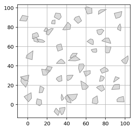
Example
from polygon_maze_generator import PolygonMazeGenerator as PMG

obstacles = []
spacing = 15
for x in range(0, 100, spacing):
    for y in range(0, 100, spacing):
        offset = np.random.randn(2) * 5
        obstacles.append(PMG.create_convex() + np.array([x, y]) + offset)
PMG.save_svg(obstacles, "test.svg")
PMG.plot(obstacles)
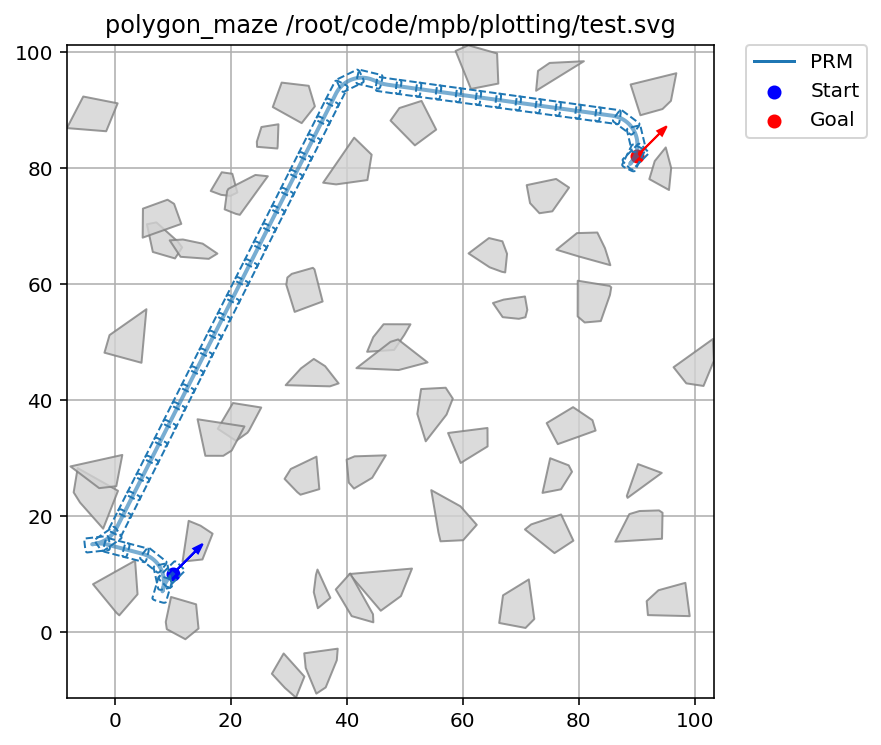
Use MPB.set_polygon_env(svg_filename) to set the SVG file as environment for the given MPB instance.
m = MPB()
m["max_planning_time"] = 30
m.set_start(10., 10., 45 * np.pi / 180)
m.set_goal(90., 82., 45 * np.pi / 180)
m.set_polygon_env(os.path.abspath("test.svg"))
m.set_planners(['prm'])
if m.run(id="test", runs=1) == 0:
    m.visualize_trajectories(draw_start_goal_thetas=True, plot_every_nth_polygon=10, silence=True)
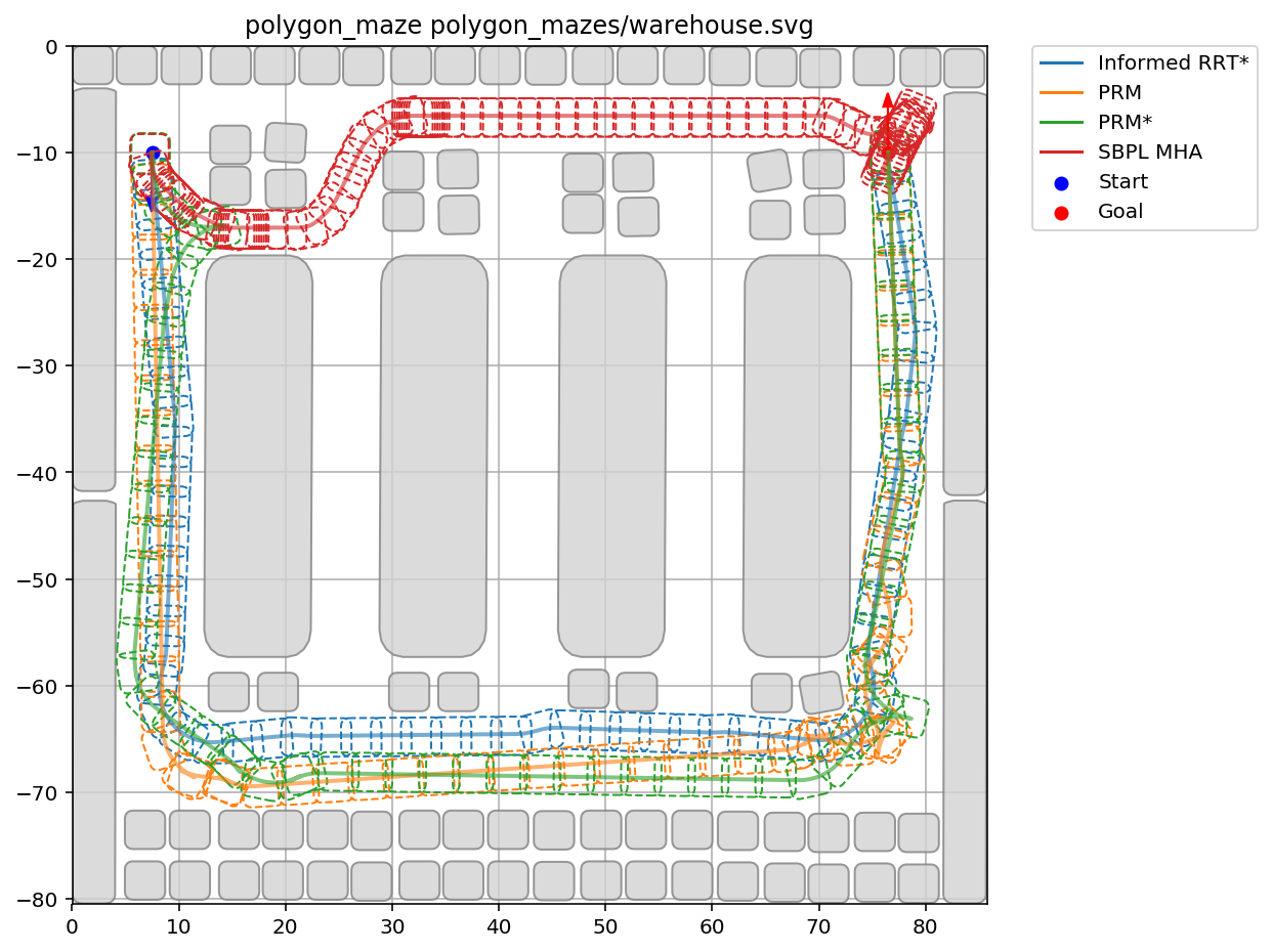
Load Maze from SVG File
The following example demonstrates how to run several planners on the warehouse polygon-based environment, which constitutes one of the images in Figure 1 of our paper.
In this example, the collision shape of the robot is also changed to warehouse_robot.svg.
Example
m = MPB()
scenario = "warehouse"
m["max_planning_time"] = 30
m["env.start"] = {"theta": -1.58, "x": 7.5, "y": -10}
m["env.goal"] = {"theta": 1.58, "x": 76.5, "y": -10}
m["env.type"] = "polygon"
m.set_polygon_env("polygon_mazes/%s.svg" % scenario)
m["env.collision.robot_shape_source"] = "polygon_mazes/warehouse_robot.svg"
m.set_planners([])
m.set_planners(['bfmt', 'cforest', 'prm', 'prm_star', 'informed_rrt_star', 'sbpl_mha'])
m["steer.car_turning_radius"] = 2
m["sbpl.scaling"] = 1
m.run(id="test_%s" % scenario, runs=1)
Visualize the trajectories:
m.visualize_trajectories(ignore_planners='cforest, bfmt',
                         draw_start_goal_thetas=True,
                         plot_every_nth_polygon=8,
                         fig_width=8,
                         fig_height=8,
                         silence=True,
                         save_file="plots/%s.pdf" % scenario,
                         num_colors=10)